Lesson 1 of 6 · Building language models
A language model made of counts
After “bug is,” what word comes next? Look for those two words in the training text and count what followed. This small model uses those observed fractions as its next-word probabilities.
Our teaching model: ordinary tokens are words, and the context is the previous two tokens. Modern LLMs usually use finer-grained text tokens and learn probabilities with neural networks. Here we make the calculation visible.
Start with the evidence
Edit the text. Watch the probabilities change.
The training text supplies examples to learn from. The context is the preceding text we use to predict a next token. Start with “bug is”: which lines contain it, and what followed each time?
The default model uses the last two tokens. Clear this field to predict the beginning of a sequence.
Change context length or sequence boundaries
An n-gram's name counts the context plus the target: a trigram uses two preceding tokens, a bigram one, and a unigram none.
Separate sequences have their own start/end markers. A single passage can form context/target rows across line breaks. The text can be long while each prediction still uses a short context.
Next-token probabilities
| Next token | Count / matches | Probability |
|---|
Where these counts came from
| Training occurrence | Context | Following token |
|---|
Inspect all training rows
Each row uses the context from the supplied training text and the token that actually followed it. Repeated occurrences each contribute a count. Boundary markers are explained below.
| Sequence / target | Context | Target |
|---|
1 · Explain the result
Two of four observations becomes a 50% estimate
In the original five lines, “bug is” appears four times. Its following tokens are urgent, urgent, reproducible, broken. The repeated sentence counts twice because it occurs twice in the data. “The build is broken” has a different context, so it contributes nothing to this row.
| Following token | Matching occurrences | Estimated probability |
|---|---|---|
| urgent | 2 / 4 | 50% |
| broken | 1 / 4 | 25% |
| reproducible | 1 / 4 | 25% |
To predict after “bug is,” this count model uses those observed fractions. Building this table is what training this model does. The denominator counts matching contexts with a next-token target, not all sentences or all words in the corpus.
P(next token | context) = occurrences of context followed by that token / occurrences of context with a next-token target
Read this as “the probability of this next token, given this context.” It estimates future text from the sample; it does not guarantee what a person will write or tell us whether a claim is true.
Try the edit above: add another “the bug is broken.” There are now five matches: urgent twice, broken twice, reproducible once. The probabilities become 2/5, 2/5, 1/5. Urgent's count stays two, but its share falls from 50% to 40% because the denominator grew.
2 · Define the units we counted
Words are our tokens for this lesson
A token is a unit chosen by a tokenizer. We chose word tokens so you can read every count. Our tokenizer lowercases, keeps letters, digits and apostrophes inside words, and treats other punctuation as separators. It preserves accented letters.
Tokenizing the text is the first step. Preparing a complete training sequence also adds boundaries: <BOS> means beginning of sequence, and <EOS> means end of sequence.
| Step | Result |
|---|---|
| Tokenize the text | [the, bug, is, urgent] |
| Add the training boundaries | [<BOS>, <BOS>, the, bug, is, urgent, <EOS>] |
The four words are the ordinary text tokens, not the entire training sequence. The two start markers supply the first context; the model learns to predict each word and then the end marker. We will trace all five prediction targets below.
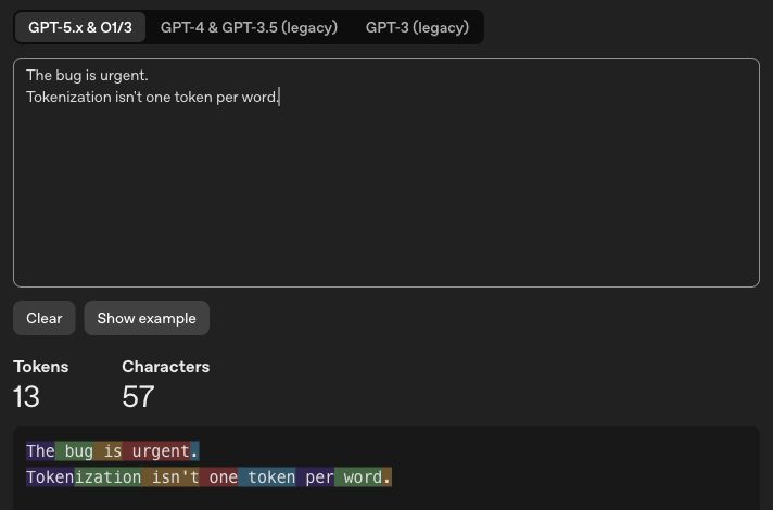
Try a real tokenizer: open the OpenAI tokenizer and enter The bug is urgent. Then try Tokenization isn't one token per word. Notice the punctuation, spaces, and word pieces. Choose the tokenizer for the model you want to inspect; different tokenizers can split the same text differently.
See the OpenAI tokenizer example
How does this differ from an LLM tokenizer?
A text tokenizer can produce whole words, word pieces, punctuation, whitespace-bearing pieces, or byte-based units. A token need not be a whole word, or even a meaningful part of one. Special tokens can mark boundaries or other model-specific structure. This lesson's word counts are not estimates of an LLM's token usage.
The vocabulary is the set of token types a model recognizes. Neural text models use integer token IDs to select learned representations. Our count table can use readable strings as dictionary keys; it does not need neural vectors. A consistent word-to-ID mapping is an equivalent representation of these same counts.
Quick check 1
Why does “the bug is urgent” contain four ordinary tokens here?
3 · Turn text into training rows
Learn how to start, continue, and stop
A trigram uses two context tokens to predict a third, the target. Slide that context through the supplied text. During training the target is the token that actually followed, not a token generated by the model.
At the beginning, we have no words yet. Our convention supplies two <BOS> (beginning-of-sequence) markers. We also append one <EOS> (end-of-sequence) target so the model learns to stop. These are reserved markers; BOS is not an empty string or generic batch padding.
Complete rows for “the bug is urgent”
| Context | Target |
|---|---|
<BOS> <BOS> | the |
<BOS> the | bug |
the bug | is |
bug is | urgent |
is urgent | <EOS> |
The first row learns a first word; the second learns what follows the first word; the last learns when the sequence ends. With this convention, four ordinary tokens produce five prediction targets. BOS is context, not a target in this model. When we ask for a new sequence, our program supplies the starting context [<BOS>, <BOS>]. The model predicts the first word from it. When the model selects EOS, our program stops generation.
Every nonempty training sequence contributes its beginning and ending. We reuse the same reserved BOS and EOS token types each time; we do not invent a new token ID for every sentence. Their repeated occurrences accumulate counts just like words do. In the original five lines, the first target is always “the,” so it has five of five matches after [<BOS>, <BOS>]. Those five sequences supply 25 training rows in total, including five EOS targets.
What if some sequences start differently or continue longer?
Start with the original five lines, then add a bug is urgent again as a sixth line in the workbench. Now the same start markers lead to two possible first words, and “is urgent” can lead either to EOS or another word:
| Context | Next token | Estimated probability |
|---|---|---|
<BOS> <BOS> | a | 1 / 6 |
<BOS> <BOS> | the | 5 / 6 |
is urgent | <EOS> | 2 / 3 |
is urgent | again | 1 / 3 |
Clear the prediction context to inspect the first-word probabilities. Then enter is urgent to inspect the choice between stopping and continuing. These estimates come from the beginnings and endings in the training text, using exactly the same counting rule as every other prediction.
This is our explicit boundary convention. Other models and training pipelines can use different boundary or packing rules.
Quick check 2
For the one sentence “the bug is urgent,” how many context → target training samples does our two-BOS, one-EOS model produce?
Count the prediction targets in the complete table above. One input sentence can supply several training samples.
4 · Use the same process on longer text
A long passage supplies many short training rows
Training text does not have to come in four-word sentences. One long passage supplies a next-token target at each word and at its end. Every occurrence of a context contributes, including repeated occurrences within the same passage. A larger corpus gives us more observations; this trigram still reads only the previous two tokens for each prediction.
Our workbench initially treats each line as a separate sequence. In “Change context length or sequence boundaries,” choose one long passage to allow rows across line breaks. Joining red bird and blue sky creates [red, bird] → blue; keeping them separate gives the first sequence an end target instead. Boundaries change the data the model learns.
The Shakespeare exercise counts through a Hamlet excerpt as one sequence, including its line breaks. The same method can read a much longer supplied text. Separate works can retain their own boundaries.
Quick check 3 · Explain the evidence
In the original corpus, why is P(urgent | bug is) = 50%?
5 · See what the evidence cannot tell us
“Never observed” becomes zero—or no estimate
For a known context, this first version uses only the continuations we counted. In the original corpus, “build” never followed “bug is,” so its probability there is 0/4. That does not prove the continuation is impossible; it means our sample did not contain it.
Now query is the in the workbench. Both words are known, but this ordered pair never appears. There are no matching observations to divide by, so this version returns no estimate. It does not return a valid distribution with every probability set to zero.
These direct count fractions are called unsmoothed estimates: we have not adjusted them to allow for missing observations. Separately, our program has no fallback to shorter contexts. Those are two choices of this implementation.
How could smoothing or backoff help?
Smoothing adjusts the estimates to reserve probability for continuations the sample missed. It addresses “not observed” versus “impossible”; it does not mean drawing a smoother curve or learning word meanings.
For example, add-one smoothing gives every possible output token one extra, assumed count. In our original corpus there are seven ordinary word types plus EOS: eight possible outputs. After “bug is,” the denominator becomes 4 + 8 = 12. Urgent gets 3/12, broken and reproducible each get 2/12, and each of the other five tokens gets 1/12. The training observations have not changed. We moved probability to unobserved outcomes while keeping the total at one.
This deliberately simple adjustment can give unseen outcomes too much probability. Other methods adjust counts more carefully. Smoothing is established in n-gram modeling, but it is not automatically how a neural LLM estimates its probabilities.
Backoff uses a shorter context when the longer one lacks evidence. For an unseen two-word context ending in “is,” a defined fallback could count what followed “is” alone. In our five sentences: urgent twice, broken twice, reproducible once → 40%, 40%, 20%. The build sentence now contributes because it matches this shorter context. Another method, interpolation, combines estimates from different context lengths.
The workbench keeps direct counts and no fallback so every probability is traceable to its matching observations. Smoothing and backoff are optional extensions, not controls secretly active in this example. An entirely new word also needs a vocabulary policy; smoothing does not invent a token representation.
6 · Use the trained table
Predict, append, and repeat until EOS
Start with an empty history, choose a next token using its distribution, append it, and look up the next context. Stop when EOS is selected. During generation the context includes earlier model outputs; during training the contexts came from the supplied text.
This trace uses your current workbench text and model order. Choosing the most likely token and sampling according to the probabilities are different ways to use the same table. Neither changes its counts.
| Context used | Token chosen | Its probability |
|---|
A 30-step limit prevents an endless loop. Reaching that limit or an unseen context is different from the model choosing EOS.
counts[context][next_token] += 1
# For an observed context:
total = sum(counts[context].values())
probability = counts[context][candidate] / total
Download the complete count model. Run it with Python 3.10 or later; the basic example needs only the standard library. It prints all 25 training rows, the probabilities, and a generation trace. An unseen context returns an empty result instead of dividing by zero.
Download the full Python bundle for optional NumPy experiments and charts. The count model above runs on its own. Setup instructions.
Your turn
Explain it in your own words.
In the original training text, why does this model give ‘urgent’ a 50% probability after ‘bug is’? Then add one more ‘the bug is broken’ line. Give the three new next-token probabilities and explain why urgent's probability changes even though its count does not.
Answer the question in your own words. A short explanation is enough.
Your feedback
Work through a hint
Hint 1
Find every occurrence of the exact context bug is and read the following token. Does the build sentence match this context?
Hint 2
The added line contributes one more broken target and one more matching context. Urgent's count stays two; what happens to its denominator?
A worked explanation
Urgent followed two of the four original bug is occurrences, so its estimate was 2/4. The added broken example makes five matches: urgent 2/5, broken 2/5, reproducible 1/5. Urgent's share falls because the denominator grew.